Estimating wireless range usually means juggling a spreadsheet of link-budget numbers and a separate propagation model, then guessing at the noise floor and the fade margin. Change the modulation and you retype the sensitivity. Change the environment and you swap the path-loss exponent by hand.
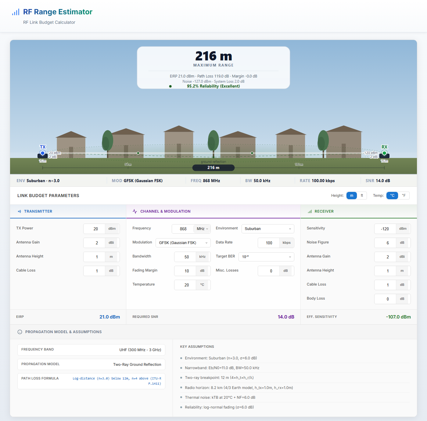
The Salitronic RF Link Budget Calculator does the whole chain at once. Pick a modulation or protocol, a frequency, and an environment, and it computes the EIRP, the thermal noise floor, the required SNR, the effective receiver sensitivity, the path loss, the link margin, the reliability, and the resulting maximum range — and draws the link as a physics-accurate cross-section. All in one browser tab, free, no signup. Nothing leaves your machine.
What It Does
Full Link Budget
One pass from transmitter to receiver: EIRP (TX power + antenna gain − cable loss), path loss at range, system losses (cable, body, misc), fade margin, and the link margin. The result is the maximum range in metres, kilometres and miles, with the dominant terms shown so you can see exactly where the budget is spent.
Protocols & Modulations
Forty-plus presets: LoRa SF7–SF12, BLE 1M / 2M / Coded S2 / S8, Zigbee / 802.15.4, Wi-Fi 802.11b and 5 GHz, Sigfox uplink/downlink, Z-Wave, Wireless M-Bus, DECT, ANT, PMR446, and the generic building blocks OOK, ASK, FSK, GFSK, MSK, GMSK, BPSK, QPSK, 8-PSK, 16/64-QAM. Each protocol carries its published datasheet sensitivity; the generic modulations compute sensitivity from Eb/N0 and your bandwidth and data rate.
Propagation Models
The right model for the environment, switched automatically: pure Friis free-space path loss (FSPL), the two-ray ground-reflection model with breakpoint for open line-of-sight links, log-distance with empirical exponents for cluttered environments, an Egli-style antenna height-gain term for outdoor NLOS, and an ITU-R P.1238 style interior wall-penetration term for indoor links.
12 Environments
Free space, rural, suburban, urban, dense urban, indoor line-of-sight, indoor NLOS, office, industrial/warehouse, forest, over water, and mountainous terrain. Each carries a realistic path-loss exponent, log-normal shadowing sigma, and clutter loss drawn from ITU-R P.1411, COST-231 and measured data.
Noise & Sensitivity
Thermal noise floor from kTB (−174 dBm/Hz at 290 K, with a temperature correction and bandwidth), plus your receiver noise figure. Required SNR comes from the modulation's Eb/N0 at the target BER and the data-rate-to-bandwidth ratio. The effective sensitivity is the worse of the datasheet value and the computed kTB + NF + SNR figure.
Reliability & Fade Margin
A log-normal shadowing model turns your fade margin and the environment's shadowing sigma into a link-reliability percentage, so you can see how much margin a given availability actually needs in that environment.
Fresnel Zone & Horizon
First Fresnel-zone radius for line-of-sight clearance, the two-ray breakpoint distance, and the radio horizon from the 4/3-Earth model — with a clear flag when a link is limited by the horizon rather than the link budget.
Physics-Accurate Diagram
The link is drawn as a scaled cross-section of the actual environment: the signal beam, the first Fresnel zone (line-of-sight environments only, scaled with frequency), and the two-ray ground reflection (outdoor reflective ground only, with the specular point placed by antenna-height ratio). Drag either antenna to set its height and watch the range and geometry update live.
Frequency Bands
30 MHz to 10 GHz, with band-aware behaviour: VHF/UHF/SHF use the standard models, while LF/MF/HF links are range-capped with prominent warnings because ground-wave and sky-wave dominate there and log-distance no longer applies. SHF links carry a rain-fade caution.
Units & Transparency
Metres or feet, °C or °F, kHz / MHz / GHz. Every result is accompanied by the propagation model used and the list of assumptions behind it, so the number is never a black box. Protocols lock to their real operating frequency automatically (BLE to 2.4 GHz, DECT to 1.9 GHz, and so on).
The Physics Is Validated
The propagation and link-budget maths are checked, not hand-waved. The two-ray model is verified against the ITU-R P.1411 line-of-sight envelope; the modulation Eb/N0 figures are the textbook per-bit values at the target BER; the LoRa sensitivities match the Semtech SX1276 datasheet per spreading factor; and the predicted ranges are cross-checked against published field measurements for LoRa, BLE, Zigbee, Wi-Fi, Sigfox and ISM links. Free space is the true ideal (pure Friis, no ground), so it is the theoretical best case the other models sit below.
Who Uses It
- Firmware and hardware engineers sizing a wireless link before committing to a radio or an antenna.
- IoT and LoRaWAN deployers estimating gateway coverage across rural, suburban and urban sites.
- Product teams comparing protocols — BLE vs LoRa vs Sigfox — for range against data rate and power.
- RF and systems engineers sanity-checking a link budget against the noise floor, fade margin and sensitivity.
- Students and educators learning path loss, link budgets, Fresnel zones and the two-ray model with a tool that shows its working.
Frequently Asked Questions
What does it calculate?
The maximum range of a wireless link, plus the full chain behind it: EIRP, path loss at range, thermal noise floor, required SNR, effective receiver sensitivity, link margin, link reliability, the first Fresnel-zone radius, the two-ray breakpoint, and the radio horizon. It also shows the range-vs-distance signal profile and a scaled diagram of the link in its environment.
Which protocols and modulations are supported?
LoRa (SF7–SF12), BLE (1M, 2M, Coded S2/S8), Zigbee/802.15.4, Wi-Fi 802.11b and 5 GHz, Sigfox, Z-Wave, Wireless M-Bus, DECT, ANT, PMR446, the ISM-band FSK presets, and the generic modulations OOK, ASK, FSK, GFSK, MSK, GMSK, BPSK, QPSK, O-QPSK, 8-PSK, 16-QAM and 64-QAM. Datasheet-spec protocols use their published sensitivity; generic modulations compute it from Eb/N0, bandwidth and data rate.
Which propagation models does it use?
Pure Friis free-space path loss for the ideal case; the two-ray ground-reflection model with a breakpoint for open line-of-sight links; a log-distance model with environment-specific exponents and clutter for cluttered outdoor and indoor links; an Egli-style height-gain term for outdoor NLOS; and an ITU-R P.1238 style wall-penetration term indoors. The tool picks the appropriate model from the chosen environment and always tells you which one it used.
Does antenna height matter?
It depends on the environment. In free space there is no ground plane, so height has no effect and the height control is disabled (pure FSPL is a function of distance and frequency only). For outdoor line-of-sight environments, height drives the two-ray ground reflection and the breakpoint; for outdoor NLOS, raising the antenna above the clutter increases range via the height-gain term. Indoors, height is bounded by the ceiling.
How accurate is it?
It is a theoretical estimate based on standard propagation models, validated against ITU-R recommendations and published field measurements, and it is intentionally conservative (it applies a fade margin and clutter loss). Real range depends on the specific terrain, obstacles, interference, antenna patterns and weather, so treat the result as a well-grounded starting point and confirm with field tests.
What frequency range does it cover?
30 MHz to 10 GHz. VHF, UHF and SHF use the standard models. Below 30 MHz (LF/MF/HF) the result is range-capped with prominent warnings, because ground-wave and sky-wave propagation dominate there and the log-distance model is not valid.
Are my inputs uploaded to a server?
No. The calculation runs entirely in your browser as a WebAssembly module. Nothing you type is sent anywhere.
Is there an API or downloadable version?
Not currently — the tool is web only. If you need batch calculation or integration, reach out via the contact page.